Generating difficult Sudoku puzzles quickly
13 Jun 2011
This article explains a simple method to quickly estimate the difficulty of a Sudoku puzzle which correlates reasonably well with human estimates of difficulty. It also gives an algorithm which can be used to generate difficult puzzles reliably and efficiently. Source code for an implementation of this algorithm is also provided.
In the following, the time complexities are specified with N being the width/height of the grid (9 for regular Sudoku).
Solver
The basic approach to solving a Sudoku puzzle is by a backtracking search of candidate values for each cell. The general procedure is as follows:
Generate, for each cell, a list of candidate values by starting with the set of all possible values and eliminating those which appear in the same row, column and box as the cell being examined.
Choose one empty cell. If none are available, the puzzle is solved.
If the cell has no candidate values, the puzzle is unsolvable.
For each candidate value in that cell, place the value in the cell and try to recursively solve the puzzle.
There are two optimizations which greatly improve the performance of this algorithm:
When choosing a cell, always pick the one with the fewest candidate values. This reduces the branching factor. As values are added to the grid, the number of candidates for other cells reduces too.
When analysing the candidate values for empty cells, it’s much quicker to start with the analysis of the previous step and modify it by removing values along the row, column and box of the last-modified cell. This is O(N) in the size of the puzzle, whereas analysing from scratch is O(N3).
In order to solve a puzzle, we normally terminate the algorithm once a valid solution is found or the search tree is exhausted. However, for generating puzzles we need a solver which continues after finding a valid solution. The modified solver terminates when the search tree is exhausted, or when at least two solutions have been found. We can then distinguish between three cases:
- Unsolvable.
- Solvable, but not uniquely.
- Uniquely solvable.
For a puzzle to be valid, it must be uniquely solvable.
Difficulty estimation
Estimating the difficulty of a Sudoku puzzle is a tricky problem because of the variety of techniques human solvers use. A quick and easy method that correlates roughly with difficulty is to keep track of the branch factor at each step on the path from the root of the search tree to the solution.
We compute a branch-difficulty score by summing (Bi - 1)2 at each node, where Bi are the branch factors. A solution which requires no backtracking at all would thus have a branch-difficulty score of 0.
The final score is given by:
S = B * 100 + EWhere B is the branch-difficulty score and E is the number of empty cells. E is included to bias the puzzle generator in the direction of fewer clues, given multiple puzzles with the same branch-difficulty.
A puzzle which requires no backtracking ends up with a final score of less than 100. However, this naive approach does not correlate well with actual difficulty unless a modification is made to the solver algorithm. This is described in the next section.
Set-oriented freedom analysis
The solver described above does well when the puzzle contains naked singles, requiring no backtracking. It also does well with naked tuples, giving branching factors of 2 for naked pairs, 3 for naked triples, and so on.
However, there is a simple technique used by human solvers to simplify puzzles which is completely missed by this algorithm. Rather than considering the possible values for a given empty cell, we could consider possible positions for a given missing value in one of the rows, columns or boxes.
We make the following modification to the solver:
Choose the cell with the fewest possible candidates. If no such cell can be found, the puzzle is solved.
Search sets (rows, columns and boxes) for missing values, and count the positions they could occupy. Identify the set and value with the fewest number of possible positions.
If the set-search result gives a number of positions which is smaller than the number of candidate values found in step 1, then continue with step 4. Otherwise, continue with step 5.
Try filling the identified value in each candidate position in the set and recursively solve. If all candidate positions are exhausted, signal failure to the caller.
For each candidate value in the cell identified in step 1, place the value in the cell and try to recursively solve the puzzle. If all candidate values are exhausted, signal failure.
Essentially, the algorithm is the same, except that we try the set-oriented approach if it results in a smaller branch factor. This means that hidden singles or tuples yield similar branch factors to their naked equivalents.
Making this modification often changes the results of difficulty estimations drastically. Consider this puzzle as an example:
╔═══╤═══╤═══╦═══╤═══╤═══╦═══╤═══╤═══╗
║ 5 │ 3 │ 4 ║   │   │ 8 ║   │ 1 │   ║
╟───┼───┼───╫───┼───┼───╫───┼───┼───╢
║   │   │   ║   │   │ 2 ║   │ 9 │   ║
╟───┼───┼───╫───┼───┼───╫───┼───┼───╢
║   │   │   ║   │   │ 7 ║ 6 │   │ 4 ║
╠═══╪═══╪═══╬═══╪═══╪═══╬═══╪═══╪═══╣
║   │   │   ║ 5 │   │   ║ 1 │   │   ║
╟───┼───┼───╫───┼───┼───╫───┼───┼───╢
║ 1 │   │   ║   │   │   ║   │   │ 3 ║
╟───┼───┼───╫───┼───┼───╫───┼───┼───╢
║   │   │ 9 ║   │   │ 1 ║   │   │   ║
╠═══╪═══╪═══╬═══╪═══╪═══╬═══╪═══╪═══╣
║ 3 │   │ 5 ║ 4 │   │   ║   │   │   ║
╟───┼───┼───╫───┼───┼───╫───┼───┼───╢
║   │ 8 │   ║ 2 │   │   ║   │   │   ║
╟───┼───┼───╫───┼───┼───╫───┼───┼───╢
║   │ 6 │   ║ 7 │   │   ║ 3 │ 8 │ 2 ║
╚═══╧═══╧═══╩═══╧═══╧═══╩═══╧═══╧═══╝
With the naive solver algorithm, the difficulty score given was 655, indicating that the solver may have backtracked multiple times. However, the modified solver allocated a score of only 55. No backtracking was necessary. In the cases where the original solver backtracked, cells could be filled with certainty by identifying hidden singles.
Scores of less than 100 indicate easy puzzles with no backtracking required. Scores in the 300+ range are usually fairly challenging and require at least the elimination of hidden/naked tuples, and sometimes more advanced techniques such as forcing chains.
Grid generator
The first step in generating a puzzle is to produce a valid solution grid. The easiest method of doing this is a variation on the naive backtracking solver. To fill the grid, we apply this algorithm:
Choose the empty cell with the fewest possible candidates. If no such cell exists, the grid is filled and the algorithm should terminate.
Choose a candidate at random and place it in the cell. Try to recursively fill the grid. If this fails, choose a different candidate at random and retry.
If all candidates are exhausted, signal failure to the caller.
It’s important that candidates are picked in random order - otherwise we end up with the same solution grid each time.
Optimization
To speed up the grid generator, we can fill the top band and the first column without backtracking. Starting with an empty grid, the upper-left box can always be filled with any permutation of the digits 1 to 9, as there are no constraints yet imposed. We might end up with:
╔═══╤═══╤═══╦═══╤═══╤═══╦═══╤═══╤═══╗
║ 2 │ 8 │ 4 ║   │   │   ║   │   │   ║
╟───┼───┼───╫───┼───┼───╫───┼───┼───╢
║ 3 │ 7 │ 9 ║   │   │   ║   │   │   ║
╟───┼───┼───╫───┼───┼───╫───┼───┼───╢
║ 5 │ 1 │ 6 ║   │   │   ║   │   │   ║
╠═══╪═══╪═══╬═══╪═══╪═══╬═══╪═══╪═══╣
.....................................
The top-middle box can be filled next, but it gets slightly complicated. Initially, there are 6 candidates each for the three box-row tuples. After choosing three for the top box-row, the choices for the next two box-rows may be limited. For example, if we were to choose the tuple (3, 7, 9) to fill the top box-row in the example above, the choices for the next two box-rows would be restricted to (1, 5, 6) and (2, 4, 8) respectively. We need to terminate the selection of values for the second box-row early if the set of candidates for the bottom box-row is reduced to three.
After choosing three tuples for the box-rows in the middle box, they can be permuted randomly into each box-row:
╔═══╤═══╤═══╦═══╤═══╤═══╦═══╤═══╤═══╗
║ 2 │ 8 │ 4 ║ 9 │ 3 │ 6 ║   │   │   ║
╟───┼───┼───╫───┼───┼───╫───┼───┼───╢
║ 3 │ 7 │ 9 ║ 1 │ 5 │ 8 ║   │   │   ║
╟───┼───┼───╫───┼───┼───╫───┼───┼───╢
║ 5 │ 1 │ 6 ║ 7 │ 2 │ 4 ║   │   │   ║
╠═══╪═══╪═══╬═══╪═══╪═══╬═══╪═══╪═══╣
.....................................
The tuples top-right box are determined for each box-row by the other 6 values in the row. In this case, they are (1, 5, 7), (2, 4, 6) and (3, 8, 9). All that remains is to randomly permute them within each box-row:
╔═══╤═══╤═══╦═══╤═══╤═══╦═══╤═══╤═══╗
║ 2 │ 8 │ 4 ║ 9 │ 3 │ 6 ║ 1 │ 5 │ 7 ║
╟───┼───┼───╫───┼───┼───╫───┼───┼───╢
║ 3 │ 7 │ 9 ║ 1 │ 5 │ 8 ║ 6 │ 4 │ 2 ║
╟───┼───┼───╫───┼───┼───╫───┼───┼───╢
║ 5 │ 1 │ 6 ║ 7 │ 2 │ 4 ║ 8 │ 9 │ 3 ║
╠═══╪═══╪═══╬═══╪═══╪═══╬═══╪═══╪═══╣
.....................................
At this point, there are three values already used in the first column. We can randomly permute the remaining 6 along the remaining empty cells in the first column, leaving only 48 of the 81 total cells to be filled by the backtracking grid filler.
Puzzle generator
Given a valid solution grid, the final task is to generate a puzzle by clearing cells, leaving enough clues to guarantee that the puzzle is uniquely solvable. We do this by a random search over the space of possible puzzles with the given solution. A naive strategy for this would be:
Start by storing the solution grid as the best puzzle, with a score of 0.
Randomly add or remove a pair of clues from the grid.
If the new grid is uniquely solvable, with a higher score than the best puzzle so far, store it as the new best puzzle.
Repeat steps 2 and 3 for as many iterations as desired.
The main problem with this approach is that it can get stuck in local maxima in the search space. To rememdy this, we allow the search to wander for 20 random steps from the starting grid before starting the next iteration from the best puzzle found so far.
Implementation and results
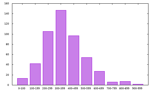
Implementing this algorithm and testing by generating 500 random puzzles (200 iterations each) yielded the following distribution of puzzle difficulty scores:
On a 1.66 GHz Atom N450, these puzzles take on average 596 ms to generate.
The source for the puzzle generator is here. Compile with:
gcc -O3 -Wall -o sugen sugen.cTo generate a puzzle:
./sugen -u generateType sugen --help for more options.
Sample puzzles
The following puzzles were generated by the above program. The difficulty scores are listed below each puzzle:
╔═══╤═══╤═══╦═══╤═══╤═══╦═══╤═══╤═══╗  ╔═══╤═══╤═══╦═══╤═══╤═══╦═══╤═══╤═══╗
║ 3 │ 7 │   ║   │   │ 9 ║   │   │ 6 ║  ║   │ 7 │   ║ 3 │   │   ║   │ 4 │   ║
╟───┼───┼───╫───┼───┼───╫───┼───┼───╢  ╟───┼───┼───╫───┼───┼───╫───┼───┼───╢
║ 8 │   │   ║ 1 │   │ 3 ║   │ 7 │   ║  ║ 3 │   │   ║   │ 8 │   ║ 2 │   │   ║
╟───┼───┼───╫───┼───┼───╫───┼───┼───╢  ╟───┼───┼───╫───┼───┼───╫───┼───┼───╢
║   │   │   ║   │   │   ║   │   │ 8 ║  ║ 2 │   │ 1 ║ 4 │   │ 7 ║   │   │   ║
╠═══╪═══╪═══╬═══╪═══╪═══╬═══╪═══╪═══╣  ╠═══╪═══╪═══╬═══╪═══╪═══╬═══╪═══╪═══╣
║   │ 2 │   ║   │ 8 │   ║   │   │ 5 ║  ║ 5 │   │ 4 ║   │   │   ║   │ 9 │   ║
╟───┼───┼───╫───┼───┼───╫───┼───┼───╢  ╟───┼───┼───╫───┼───┼───╫───┼───┼───╢
║ 1 │ 8 │ 7 ║   │   │   ║ 6 │ 4 │ 2 ║  ║   │ 2 │   ║   │   │   ║   │ 5 │   ║
╟───┼───┼───╫───┼───┼───╫───┼───┼───╢  ╟───┼───┼───╫───┼───┼───╫───┼───┼───╢
║ 5 │   │   ║   │ 2 │   ║   │ 1 │   ║  ║   │ 1 │   ║   │   │   ║ 7 │   │ 3 ║
╠═══╪═══╪═══╬═══╪═══╪═══╬═══╪═══╪═══╣  ╠═══╪═══╪═══╬═══╪═══╪═══╬═══╪═══╪═══╣
║ 7 │   │   ║   │   │   ║   │   │   ║  ║   │   │   ║ 9 │   │ 6 ║ 3 │   │ 2 ║
╟───┼───┼───╫───┼───┼───╫───┼───┼───╢  ╟───┼───┼───╫───┼───┼───╫───┼───┼───╢
║   │ 5 │   ║ 6 │   │ 2 ║   │   │ 7 ║  ║   │   │ 2 ║   │ 3 │   ║   │   │ 9 ║
╟───┼───┼───╫───┼───┼───╫───┼───┼───╢  ╟───┼───┼───╫───┼───┼───╫───┼───┼───╢
║ 2 │   │   ║ 3 │   │   ║   │ 6 │ 1 ║  ║   │ 6 │   ║   │   │ 2 ║   │ 8 │   ║
╚═══╧═══╧═══╩═══╧═══╧═══╩═══╧═══╧═══╝  ╚═══╧═══╧═══╩═══╧═══╧═══╩═══╧═══╧═══╝
Difficulty: 551                        Difficulty: 253

╔═══╤═══╤═══╦═══╤═══╤═══╦═══╤═══╤═══╗  ╔═══╤═══╤═══╦═══╤═══╤═══╦═══╤═══╤═══╗
║   │ 4 │   ║   │   │ 7 ║   │ 9 │   ║  ║   │   │ 3 ║   │   │   ║   │   │   ║
╟───┼───┼───╫───┼───┼───╫───┼───┼───╢  ╟───┼───┼───╫───┼───┼───╫───┼───┼───╢
║   │ 9 │ 1 ║   │ 8 │   ║   │   │   ║  ║ 8 │   │ 9 ║ 4 │ 6 │   ║ 7 │   │ 2 ║
╟───┼───┼───╫───┼───┼───╫───┼───┼───╢  ╟───┼───┼───╫───┼───┼───╫───┼───┼───╢
║ 7 │   │ 3 ║ 9 │   │ 1 ║   │   │   ║  ║ 2 │   │   ║   │ 1 │ 8 ║ 6 │   │   ║
╠═══╪═══╪═══╬═══╪═══╪═══╬═══╪═══╪═══╣  ╠═══╪═══╪═══╬═══╪═══╪═══╬═══╪═══╪═══╣
║   │ 1 │   ║   │ 6 │ 4 ║ 2 │   │   ║  ║   │   │   ║   │   │ 6 ║   │ 7 │   ║
╟───┼───┼───╫───┼───┼───╫───┼───┼───╢  ╟───┼───┼───╫───┼───┼───╫───┼───┼───╢
║   │   │   ║ 5 │   │ 8 ║   │   │   ║  ║   │   │ 8 ║   │   │   ║ 4 │   │   ║
╟───┼───┼───╫───┼───┼───╫───┼───┼───╢  ╟───┼───┼───╫───┼───┼───╫───┼───┼───╢
║   │   │ 5 ║ 7 │ 1 │   ║   │ 6 │   ║  ║   │ 7 │   ║ 8 │   │   ║   │   │   ║
╠═══╪═══╪═══╬═══╪═══╪═══╬═══╪═══╪═══╣  ╠═══╪═══╪═══╬═══╪═══╪═══╬═══╪═══╪═══╣
║   │   │   ║ 1 │   │ 5 ║ 8 │   │ 6 ║  ║   │   │ 2 ║ 9 │ 4 │   ║   │   │ 5 ║
╟───┼───┼───╫───┼───┼───╫───┼───┼───╢  ╟───┼───┼───╫───┼───┼───╫───┼───┼───╢
║   │   │   ║   │ 4 │   ║ 9 │ 1 │   ║  ║ 4 │   │ 6 ║   │ 3 │ 2 ║ 8 │   │ 7 ║
╟───┼───┼───╫───┼───┼───╫───┼───┼───╢  ╟───┼───┼───╫───┼───┼───╫───┼───┼───╢
║   │ 5 │   ║ 8 │   │   ║   │ 2 │   ║  ║   │   │   ║   │   │   ║ 2 │   │   ║
╚═══╧═══╧═══╩═══╧═══╧═══╩═══╧═══╧═══╝  ╚═══╧═══╧═══╩═══╧═══╧═══╩═══╧═══╧═══╝
Difficulty: 451                        Difficulty: 953